In my blog yesterday (Part 1) I suggested that we could evaluate RDBMS-Hadoop integration architecture using three criteria:
How parallel are the pipes to move data between the RDBMS and the parallel file system;
Is there intelligence to push down predicates; and
Is there more intelligence to push down joins and other relational operators?
But Exadata is a split RDBMS with a parallel file system backing it… how does it measure up by these criteria?
There are effective parallel pipes between the Oracle RAC RDBMS and the Exadata Storage Subsystem… so Exadata passes the first test. Further, Exadata is smart about pushing scan and projection both down to the Storage layer.
Unfortunately there is a fairly severe imbalance between the number of nodes on the RAC side and the number of nodes on the Storage side and this creates a bottleneck. We cannot give Exadata full marks here… but as far as parallel pipes goes it stacks up pretty well.
The ability to push down predicates goes a long way towards solving this as the predicate push-down reduces the amount of data that has to move over the bottleneck. But in every data warehouse there will be queries that return lots of rows from the early execution steps… and Exadata cannot join data in the Storage Subsystem so it tries to pull data up sparingly and push down semi-joins whenever possible… it just cannot be done in every case (Note: in Exadata POCs Oracle will try to ensure that no queries are included that pull lots of data up to the RAC layer… and competitors will try to include queries that expose this weakness…).
So… Oracle also includes some intelligence to push some data down to reduce data movement. There is no way to choose to move data from the RAC layer to the Storage Subsystem and execute the query there… the Storage Subsystem can only scan and project… so again we cannot give Exadata full marks… but it is pretty smart as you will see when we start looking at alternative implementations.
Finally, Exadata cannot effectively split a single query plan across both layers… so no marks at all here.
So Exadata is pretty good… but it has weak spots that will be severe for an important set of DW queries in any implementation.
Forrester regularly provides fodder for bloggers when they report on the EDW space (see Curt Monash’s review of their last report here). They have a 2013 report out now that is quite mysterious (see here).
They report that Pivotal is up there with the leading EDW vendors and positioned to move further up.
Here is the mystery. If you go to the Pivotal site and search on “data warehouse” you get ten hits:
Eight talk about analytic data warehouses, not enterprise data warehouses;
One talks about using Hive as a data warehouse; and
One talks about data and sandboxing.
There are no hits on the term “enterprise data warehouse” and one hit on the term “EDW” which refers to why you should move data off of the EDW to an analytic platform.
As I’ve pointed out… Pivotal does not market into the EDW space. They are not developing product for that space. EDW is not part of their product strategy.
The fact that their product is a capable platform for an EDW is worth noting… and readers of this blog should consider GPDB, aka Greenplum, for EDW projects. But you should be fully aware of the risk that Pivotal is not really backing this use case.
For an analyst to suggest that Pivotal has an industry-leading strategy in a space that they are not pursuing at all is very odd.
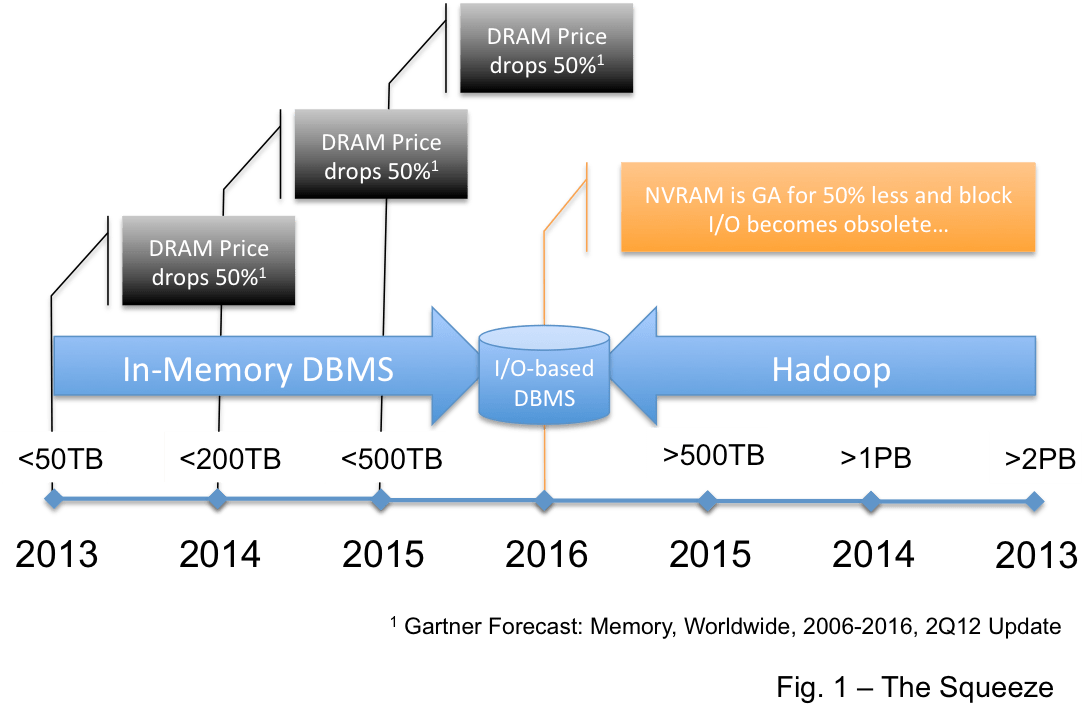
I have suggested that the big EDW parallel databases: Teradata, Exadata, Greenplum, and Netezza in particular will be squeezed over time. Colder data will move from those products to Hadoop and hotter data will move in-memory. You can see posts on this here, here, and here.
But there are three products, the Greenplum database (GPDB), HAWQ, and Aster Data, that will be squeezed more quickly as they are positioned either in between the EDW and Hadoop… or directly over Hadoop. In this post I’ll explain what I suspect Pivotal and Teradata are trying to do… why I believe their strategy will not work for long… and why readers of this blog should be careful moving forward.
The Squeeze picture assumes that Hadoop consumes more and more “big data” over time as the giant investment in that open source eco-system matures the software and improves both the performance and the feature base. I think that this is a very safe assumption. But the flip side of this assumption is that we recognize that currently the Hadoop eco-system is not particularly mature and that the performance is not top-notch. It is this flip side that provides the opportunity targeted by Pivotal and Teradata.
Here is the situation… Hadoop, even in its newbie state, is lowering the price point for biggish data. Large EDW implementations, let’s say over 100TB, that had no choice but to pick a large EDW database product 4 years ago are considering and selecting Hadoop more often at a price point 10X-20X less than the lowest street price offered by commercial DBMS vendors. But these choices are painful due to the relatively immature state of the Hadoop eco-system. It is this spot that is being targeted by Aster and GPDB… the “big data” spot where Aster and GPDB can charge a price greater than the cost of Hadoop but less than the cost of the EDW DBMS products… while providing performance and maturity worth the modest premium.
This spot, under the EDW and above Hadoop is a legitimate niche where revenue can be generated. But it is the niche that will be the first to be consumed by Hadoop as the various Hadoop RDBMS features mature. It is a niche that will not be commercially interesting in two years and will be gone in four years. Above is the Squeeze picture updated to position Aster, HAWQ and GPDB.
What would I do? Pivotal has some options. First, as I have stated before, GPDB is a solid EDW DBMS and the majority of it’s market even after running from the EDW space is there. They could move up the food chain back to the EDW space where they started and have an impact. This impact could be greater still if they could find a way to build a truly effective cloud-based EDW DBMS out of the GPDB. But this is not their current strategy and they are losing steam as an EDW both technically and in the market. The window to move back up is closing. Their current strategy which is “all-in” on Hadoop will steal business from GPDB for low-margin business around HAWQ and steal business from HAWQ for an even lower-margin business around Pivotal Hadoop. I wonder how long Pivotal can fund this strategy at a loss?
I’m not sure what I would do if I were Teradata? The investment in Aster Data is not likely to pay off before Hadoop consumes the space. Insofar as it is a sunk cost now… and they can leverage the niche described above… their positioning can earn them some revenue and stave off the full effect of the Squeeze for a short time. But Aster was never really a successful EDW play and there is no room for it to move up the food chain at Teradata.
What does this mean? Readers should take note and consider the risk that Hadoop wins in the near term… They might avoid a costly move to Aster or GPDB or HAWQ with a short lifespan. Maybe it is time to bite the bullet now and start introducing Hadoop into your infrastructure?
One final note… it is not my expectation that either the Hadoop DBMS nor any NoSQL DBMS product will consume the commercial RDBMS space anytime soon. There are reasons for this… stay tuned and I’ll post on this topic in the new year.
With this post the Database Fog Blog will receive its 100000th view. I am so grateful for your attention and consideration. And with this last post of my calendar year I wanted to say thanks… to send my regards to all whether you will be celebrating a holiday season or not… and to wish every reader, regardless of what calendar you follow, all the best in the next year…
I would like to point out a very important section in the paper on Hekaton on the Microsoft Research site here. I will quote the section in total:
2. DESIGN CONSIDERATIONS
An analysis done early on in the project drove home the fact that a 10-100X throughput improvement cannot be achieved by optimizing existing SQL Server mechanisms. Throughput can be increased in three ways: improving scalability, improving CPI (cycles per instruction), and reducing the number of instructions executed per request. The analysis showed that, even under highly optimistic assumptions, improving scalability and CPI can produce only a 3-4X improvement. The detailed analysis is included as an appendix.
The only real hope is to reduce the number of instructions executed but the reduction needs to be dramatic. To go 10X faster, the engine must execute 90% fewer instructions and yet still get the work done. To go 100X faster, it must execute 99% fewer instructions. This level of improvement is not feasible by optimizing existing storage and execution mechanisms. Reaching the 10-100X goal requires a much more efficient way to store and process data.
This is important because it confirms the difference in a Level 3 and a Level 2 columnar implementation as described here. It is just not possible for a Level 2 implementation with a row-based join engine to achieve the performance of a Level 3 implementation. This will allow the Level 3 implementations: HANA, BLU, Hekaton, and Oracle 12c to distance themselves from the Level 2 products: Teradata and Greenplum; by more than 10X… and this is a very significant advantage.
Teradata stock is falling hard due to guidance here that they may miss revenue targets. Analysts are downgrading the stock… but mostly from Buy to Neutral.
Normally stock prices would not be a relevant topic for this blog… but in this case I believe that the Squeeze I suggested first in October of 2012 and then again in February of this year (here and here) has started to affect Teradata revenues.
Note that the Squeeze should affect Netezza, Exadata, and Greenplum as well… but the effect will not be so directly reflected in the stock prices of IBM, Oracle, or EMC/VMWare/GE.
I was asked to compose a post for the SAP HANA blog to help position HANA versus the other in-memory DBs… a marketing post… not a technical post. The result here makes it clear why I am not in marketing… it sounds like someone trying too hard to be a marketeer… Still… you might like the comments…
IBM is presenting a DB2 Tech Talk that compares the BLU Accelerator to HANA. There are several mistakes and some odd thinking in the pitch so let me address the issues as a way to explain some things about HANA and about BLU. This blog will consider what data needs to be in-memory.
IBM like several others, continues to repeat a talking point along the lines of: “We believe that you should not have to fit all of you active data in memory…”. Let’s think about this…
Note that in the current release HANA has a constraint that all of the data in a single column, the entire vector that represents the data in that column, must be in-memory before it can be operated on. If the table is partitioned and partition-elimination is applied then the data in the partition for the column must be loaded in-memory. This is a real constraint that will be removed in a subsequent release… but it is not a very severe constraint if you think about it.
But let’s be clear… HANA does not require all data to be in-memory… it will read data from peripheral devices in and out as required just as BLU does.
Now what does this mean? Let’s walk through some scenarios.
First, let’s imagine a customer with 10TB of user data, per the scenario IBM discusses. Let’s not get into a whose product compresses better discussion and assume that both BLU and HANA will get 4X compression… so there is 2.5TB of user data to be processed.
Now let’s imagine a system with only a very little memory available for data. In other words, let’s configure both BLU and HANA so that they are full columnar databases, but not in-memory databases. In this case BLU would operate by doing constant I/O without constraint and HANA would fail whenever it could not fit a required column in memory. Note that HANA might not fail at all… it would depend on whether there was a large single un-partitioned column that was required.
This scenario is really silly though… HANA is an in-memory database, designed to keep data in-memory from the start… so SAP would not support this imaginary configuration. The fact that you could make BLU work out of memory is not really relevant as nowhere does IBM position, or reference, BLU as a disk-based column store add-on… you would just use DB2.
Now let’s configure a system to IBM’s specification with 400GB of memory. IBM does not really say how much of this memory is available to BLU for data… but for the sake of argument let’s ignore the system requirements and assume that BLU uses one-half, 200GB, as work space to process queries so that 200GB is available to store data in-memory. As you will see it does not really matter in this argument whether I am spot on here or not. So using IBM’s recommendation there is now a 200GB cache that can be used as data is paged in and out. Anyone who has ever used a data warehouse knows that caching does not work well for BI queries as each query touches large enough volumes of the data to flush the cache… so BLU will effectively be performing I/O for most queries and is back to being an out-of-memory columnar database. Note that this flushing issue is why the in-memory capabilities from Oracle and Teradata pin certain tables into memory. In this scenario HANA will operate exactly as BLU does with the constraint that any single column that in a compressed form exceeds 200GB will not be able to be processed.
Finally let’s configure a system with 5TB of memory per SAP’s recommendation for HANA. In this case BLU and HANA both fit all of the data in-memory… with 2.5TB of compressed user data in and 2.5TB of work space… and there is no I/O. This is an in-memory DBMS.
But according to the IBM Power 770 spec (here) there is no way to get 5TB of memory on a single p770 node… so to match HANA and eliminate all I/O they would require two nodes… but BLU cannot be deployed on a cluster… so on they would have to deploy on a single node and perform I/O on 20% of the data. The latency for SSD I/O is 200Kns and for disk it is 10Mns… for DRAM it is 100ns and HANA loads full cache lines so that the average latency is under 20ns… so the penalty paid by BLU is severe and it will never keep up with HANA.
There is more bunk around recommendations for the number of cores but I can make no sense of it at all so I do not know where to begin to debunk it. SAP recommends high-end Intel servers to run HANA. In the scenario above we would recommend multiple servers… soon enough there will be Haswell servers with 6TB of DRAM and this case will run on one node.
I have stated repeatedly that anytime a vendor presents a slide comparing their product to their competitors you should immediately throw them out… it will always be twisted. Don’t trust them. And don’t trust me as I work for SAP. But hopefully you can see some logic in my case. If you need an IMDB then you need memory. If you are short of memory then the IMDB operates like a columnar RDBMS with a memory cache. If you are running a BI query workload then you need to pin data in the cache or the system will thrash. Because of this SAP recommends that you get enough memory to get all of the data in… we recommend that you operate our in-memory database product in-memory…
This really the point of the post. The Five Minute Rule informs us about what data should be in-memory (see here). An in-memory database is designed from the bottom up to manage hot data in-memory. The in-memory add-ons being offered over legacy systems are very capable and should not be ignored… and as the price of memory drops the Five Minute Rule will suggest that data in-memory will account for and ever larger percentage of your EDW. But to offer an in-memory capability and recommend that you should keep the bulk of the data on disk is silly… and to state that your product has a competitive advantage because you do not recommend that all of the data managed by your in-memory feature be kept in-memory is silliness squared.
I recently listened to a session by Juan Loalza of Oracle on the 12c In-memory option. Here are my notes and comments in order…
There is only one copy of the data on disk and that is in row format (“the column format does not exist on disk”). This has huge implications. Many of the implications come up later in the presentation… but consider: on start-up or recovery the data has to be loaded from the row format and converted to a columnar format. This is a very expensive undertaking.
The in-memory columnar representation is a fully redundant copy of the row format OLTP representation. Note that this should not impact performance as the transaction is gated by the time to write to the log and we assume that the columnar tables are managed by MVCC just like the row tables. It would be nice to confirm this.
Data is not as compressed in-memory as in the hybrid-columnar-compression case. This is explained in my discussion of columnar compression here.
Oracle claims that an in-memory columnar implementation (level 3 maturity by my measure see here) is up to 100X faster than the same implementation in a row-based form. Funny, they did not say that the week before OOW? This means, of course, that HANA, xVelocity, BLU, etc. are 100X faster today.
They had a funny slide talking about “reporting” but explained that this is another word for aggregation. Of course in-memory vector aggregation is faster in-memory.
There was a very interesting discussion of Oracle ERP applications. The speaker suggested that there is no reporting schema for these apps and that users therefore place indexes on the OLTP database to provide performance for reporting and analytics. It was suggested that a typical Oracle E-Business table would have 10-20 indexes on it and it was not unusual to see 30-40 indexes. It was even mentioned that the Siebel application main table could require 90 indexes. It was suggested that by removing these indexes you could significantly speed up the OLTP performance, speed up reporting and analytics, cure cancer and end all wars (OK… they did not suggest that you could cure cancer and end war… this post was just getting a little dry).
The In-memory option is clusterable. Further, because a RAC cluster uses shared disk and the im-memory data is not written to disk there is a new shared-nothing implementation included. This is a very nice and significant architectural advance for Oracle. It uses the direct-to-wire infiniband protocol developed for Exadata to exchange data. Remember when Larry dissed Teradata and shared-nothingness… remember when Larry dissed in-memory and HANA… remember when Teradata dissed HANA as nonsense and said SAP was over-reacting to Oracle. Gotta smile :).
Admins need to reserve memory from the SGA for the in-memory option. This is problematic for Exadata as the maximum memory on a RAC node is 256GB… My bad… Exadata X3-8 supports 2TB of memory per node… this is only problematic for Exadata X3-2 and below… – Rob
It is possible to configure a table partition into memory while leaving other partitions in row format on disk.
It is suggested again that analytic indexes may be dropped to speed up OLTP.
The presenter talked about how the architecture, which does not change the row-based tables in any way, allows all of the high-availability options available with Oracle to continue to exist and operate unchanged.
But the beautiful picture starts to dull a little here. On start-up or first access… i.e. during recovery… the in-memory columnar data is unavailable and loaded asynchronously from the row format on disk. Note that it is possible to prioritize the order tables are loaded to get high-priority data in-memory first… a nice feature. During this time… which may be significant… all analytic queries are run against the un-indexed row store. Yikes! This kills OLTP performance and destroys analytic performance. In fact, the presenter suggested that maybe you might keep some indexes for reports on your OLTP tables to mitigate this.
Now the story really starts to unravel. Indexes are required to provide performance during recovery… so if your recovery SLA’s cannot be met without indexes then you are back to square one with indexes that are only used during recovery but must be maintained always, slower OLTP, and the extra requirement for a redundant in-memory columnar data image. I imagine that you could throttle some reports after an outage until the in-memory image is rebuilt… but the seamless operations during recovery using standard Oracle HA products is a bit of a stretch.
Let me raise again the question I asked in my post last week on this subject (here)… how are joins processed between the row format and the columnar format. The presenter says that joins are no problem… but there are really only two ways… maybe three ways to solve for this:
When a row-to-columnar join is identified the optimizer converts the columnar table to a row form and processes the join using the row engine. This would be very very slow as there would be no indexes on the newly converted columnar data to facilitate the join.
When a row-to-columnar join is identified the optimizer pushes down aggregation and projection to the columnar processing engine and converts the columnar result to a row form and processes the join using the row engine. This would be moderately slow as there would be no indexes on the newly converted columnar data to facilitate the join (i.e. the columnar fact would have no indexes to row dimensions or visa versa).
When a row-to-columnar join is identified the optimizer converts the row table to a columnar form and processes the join using the columnar engine. This could be fast.
Numbers two and three are the coolest options… but number three is very unlikely due to the fact that columnar data is sharded in a shared-nothing manner and the row data is not… and number two is unlikely because if it were the case Oracle would surely be talking about it. Number one is easy and the likely state in release 1… but these joins will be very slow.
Finally, the presenter said that this columnar processing would be implemented in Times Ten and then in the Exalytics machine. I do not really get the logic here? If a user can aggregate in their OLTP system in a flash why would they pre-aggregate data and pass it to another data stovepipe? If you had to offload workload from your OLTP system why wouldn’t you deploy a small, standard, Oracle server with the in-memory option and move data there where, as the presenter suggested, you can solve any query fast… not just the pre-aggregated queries served by Exalytics. Frankly, I’ve wondered why SAP has not marketed a small HANA server as an Exalytics replacement for just this reason… more speed… more agility… same cost?
There you have it… my half a cents… some may say cents-less evaluation.
I will end this with a question for my audience (Ofir… I’ll provide a link to your site if you post on this…)… how do we suppose the in-memory option supports bulk data load? This has implications for data warehousing…
Here, of course, is the picture I should have used above… labeled as the in-memory database of your favorite vendor:
I changed the picture to show you the billboard SAP bought on US101N right across from the O HQ…
– Rob
Larry Ellison announced a new in-memory capability for Oracle 12c last night. There is little solid information available but taken at face value the new feature is significant… very cool… and fairly capable.
In short it appears that users have the ability to pin a table into memory in a columnar format. The new feature provides level 3 (see here) columnar capabilities… data is stored compressed and processed using vector and SIMD instruction sets. The pinned data is a redundant copy of the table in-memory… so INSERT/UPDATE/DELETE and data loads queries will use the row store and data is copied and converted to the in-memory columnar format.
As you can imagine there are lots of open questions. Here are some… and I’ll try to sort out answers in the next several weeks:
It seems that data is converted row-to-columnar in real-time using a 2-phased commit. This will significantly slow down OLTP performance. LE suggested that there was a significant speed-up for OLTP based on performance savings from eliminating indexes required for analytics. This is a little disingenuous, methinks… as you will most certainly see a significant degradation when you compare OLTP performance without indexes (or with a couple of OLTP-centric indexes) and with the in-memory columnar feature on to OLTP performance without the redundant copy and format to columnar effort. So be careful. The use case suggested: removing analytic indexes and using the in-memory column store is solid and real… but if you have already optimized for OLTP and removed the analytic indexes you are likely to see performance drop.
It is not clear whether the columnar data is persisted to disk/flash. It seems like maybe it is not. This implies that on start-up or recovery data is read from the row store on-disk tables and logs and converted to columnar. This may significantly impact start-up and recovery for OLTP systems.
It is unclear how columnar tables are joined to row tables. It seems that maybe this is not possible… or maybe there is a dynamic conversion from one form to another? Note that it was mentioned that is possible for columnar data to be joined to columnar data. Solving for heterogeneous joins would require some sophisticated optimization. I suspect that when any row table is mentioned in a query that the row join engine is used. In this case analytic queries may run significantly slower as the analytic indexes will have been removed.
Because of this and of item #2 it is unclear how this feature plays with Exadata. For lots of reasons I suspect that they do not play well and that Exadata cannot use the new feature. For example, there is no mention of new extended memory options for the Exadata appliance… and you can be sure that this feature will require more memory.
There was a new hardware system announced that uses this in-memory capability… If you add all of this up it may be that this is a system designed to run SAP applications. In fact, before the presentation on in-memory there was a long (-winded) presentation of a new Fujitsu system and the SAP SD benchmark was specifically mentioned. This was not likely an accident. So… maybe what we have is a counter to HANA for SAP apps… not a data warehouse at all.
As I said… we’ll see as the technical details emerge. If the architectural constraints 1-4 above hold then this will require some work for Oracle to compete with HANA for SAP apps or for data warehouse workloads…
I posted some thoughts about HANA and OLTP here… it is pretty fair and straightforward, I hope… but as I always point out when I mention a work post on this blog… when I am there I do not promise to be objective… it is my job.


")